Why It Matters
Large-universe screening is easy to describe and expensive to run naively: take a theme, apply it to thousands of companies, split the time range into windows, and collect the Search results. That full-grid pattern is comprehensive and dependable, but it allocates the same request budget to every entity and period even when coverage is highly uneven. Smart Batching adds a planning layer before execution. It estimates where the content is likely to be, groups similar-volume entities together, splits high-volume periods more carefully, and then allocates Search budget proportionally. Standard Bigdata.com Search still does the retrieval and ranking; Smart Batching decides how to spend the requests when the universe is large.What It Does
This cookbook walks through a complete Smart Batching workflow:- Load a company universe from CSV.
- Build a reusable search plan with
plan_search(). - Execute that plan at a chosen
chunk_percentage. - Deduplicate documents and convert chunks to a DataFrame.
- Save and reload plans so different sampling levels can be tested without replanning.
- Interpret benchmark results across speed, relevance distribution, and coverage.
How It Works
Smart Batching uses a plan-then-execute flow.Step 1: Plan
plan_search() has two planning substeps:
Step 1a: Group entities into volume baskets.
The planner queries the Bigdata.com Search Volume API to estimate how many chunks each entity will produce for the topic over the full time range. It then groups entities into baskets based on expected volume: low-volume entities can be merged together, while high-volume entities can be isolated or placed in smaller baskets. This preserves the cross-sectional distribution of the universe, so companies are not flattened into a single bucket and high-coverage names do not crowd out the long tail.
Step 1b: Break each basket down by time.
For each basket, the planner pulls the expected-volume time series and partitions the full date range into batch periods. High-volume periods get shorter windows; low-volume periods can use longer windows. This preserves temporal structure in the same way Step 1a preserves cross-sectional structure: periods with heavy coverage get their own batches, and quiet periods are consolidated so execution does not spend unnecessary requests on sparse windows.
The result is a search plan with expected chunk counts and basket definitions. You can inspect it before making the larger retrieval run.
Step 2: Execute
execute_search() turns the plan into Search API calls. The chunk_percentage parameter controls the retrieval budget:
1.0requests the full planned budget.0.1requests about 10% of expected chunks per basket.0.01requests about 1% of expected chunks per basket.
1. Setup
The notebook in the cookbook repository is the best way to run the full workflow: From theSmart_Batching directory, create a local environment and install the cookbook requirements:
.env file in the Smart_Batching directory:
Imports and environment setup
Imports and environment setup
2. Configure a search
The example notebook uses a customer-confidence screen over the historical US top-company universe.3. Create a search plan
Planning estimates the expected retrieval footprint before Search execution begins. Step 1a creates volume baskets across entities, and Step 1b splits those baskets across time so both cross-sectional and temporal structure are represented. In the captured notebook run, the planner loaded 4,731 entity IDs, found chunks for 3,745 companies, estimated 69,426 chunks, and created 77 baskets.4. Execute and deduplicate
Execution runs the Search calls represented by the plan. Usechunk_percentage to select the retrieval budget.
5. Choose chunk_percentage
Treat chunk_percentage as a budget control:
- Use
0.01for alerting, LLM verification, and signal-first workflows where the highest-ranked chunks are enough. - Use
0.1for balanced research workflows, entity-level scoring, trend analysis, and dashboards. - Use
1.0when completeness matters more than latency, while still benefiting from volume-aware grouping.
6. Benchmark Results
The benchmark compared a full-grid baseline with Smart Batching at 100%, 10%, and 1% across three screening topics. Timing includes planning and execution for Smart Batching.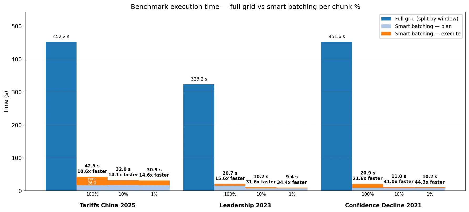
- Tariffs China 2025: full grid took 452.2 seconds. Smart Batching took 42.5 seconds at 100%, 32.0 seconds at 10%, and 30.9 seconds at 1%.
- Leadership 2023: full grid took 323.2 seconds. Smart Batching took 20.7 seconds at 100%, 10.2 seconds at 10%, and 9.4 seconds at 1%.
- Confidence Decline 2021: full grid took 451.6 seconds. Smart Batching took 20.9 seconds at 100%, 11.0 seconds at 10%, and 10.2 seconds at 1%.
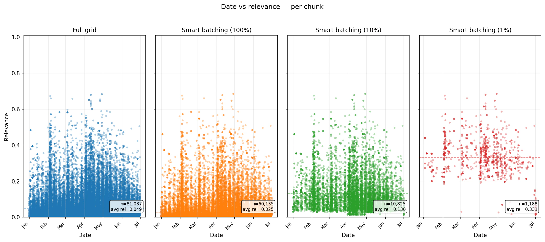
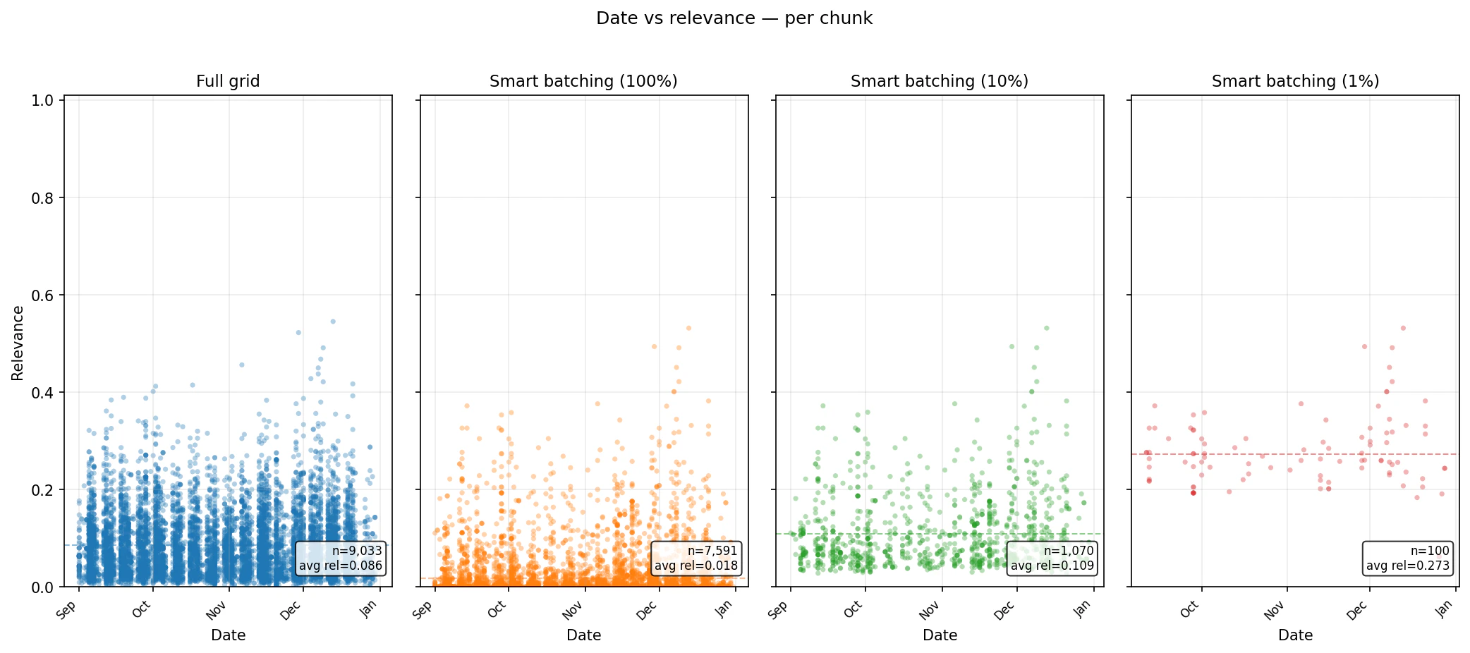
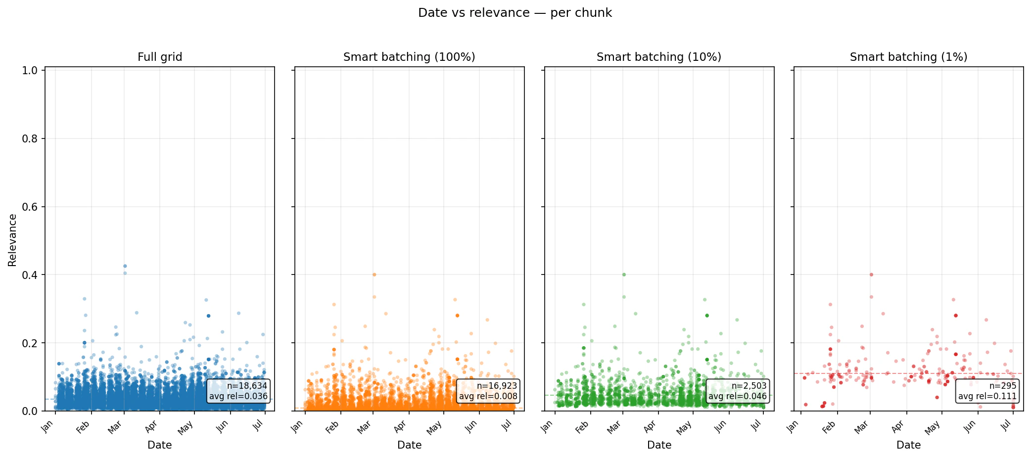
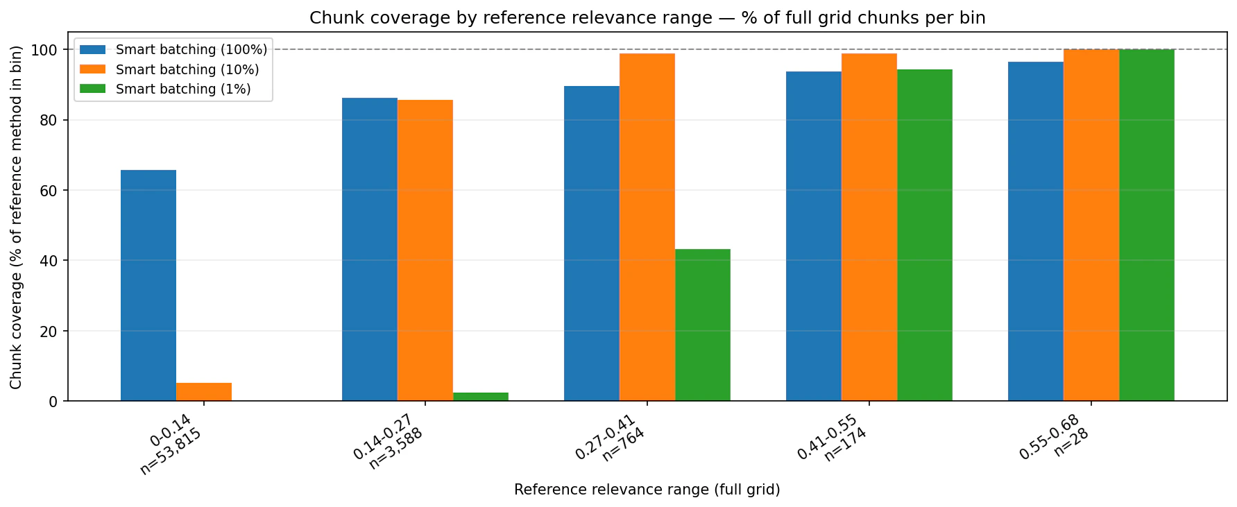
chunk_percentage settings concentrate the returned set into higher-ranked chunks while preserving date coverage.
Tariffs China 2025 — relevance distribution
Summary
Smart Batching is a practical optimization layer for large Search workflows. It keeps the retrieval quality of Bigdata.com Search, adds a planning step that understands expected volume, and gives you a direct budget control throughchunk_percentage.
For full code and a runnable notebook, see the Smart Batching folder in the bigdata-cookbook repository, especially test_smart_batching.ipynb. For direct integration, install the bigdata-smart-batching Python package.